BooleaBayes Part 2- Network Structure and Dynamics
In the first post, we took a look at why we might care about a gene regulatory network, or GRN. This post will focus on learning network structure and network dynamics.
Every network has a specific structure, determined by its combination of nodes (also known as vertices, objects, and in this case transcription factors) and edges (or connections, interactions, or effects). For the network we care about (proteins regulating genes to control cell indentity), we have a directed network, where the edges have arrows. In our network, we’ll use a single node to represent both the RNA form and protein form of a specific gene. In other words, an incoming edge to some node X will represent a transcription factor protein binding to the promoter region of the X gene, and an outgoing edge will represent the X protein binding to the promoter of another gene.
Often, researchers really only care about the structure of the network itself and can gain a lot of information from it. For example, structural controllability is concerned with the connections between nodes in the network, and how some sets of inputs are able to guide the network from any initial state to a specific, desired final state. Also, when we know which transcription factors affect others, we can look for motifs in the network, which are small patterns that tell us something about how the network will behave. Feedback loops, for example, are a common point of interest for researchers because they can drive changes in the network. A positive feedback loop is one that tends to amplify some signal, such as in blood clotting, where platelets release clotting factors that cause more platelets to aggregate at the site of injury, releasing even more factors, and so on. A negative feedback loop is one that tends to induce an opposite effect, like a thermostat regulating room temperature by comparing the actual temperature to the set temperature and adjusting (decreasing if the actual temperature is high, and vice versa). Negative feedback loops are very common in biology, as most of life functions within a relatively small range of environmental conditions (like temperature).
You might be familiar with network structure from other disciplines, such as social networks, economic networks, Google’s network of webpages, networks of airports, or even food chains and networks. In all of these cases, there will be some components with many more connections and interactions than average,* such as Atlanta’s large international airport. In the case of airports, we might call these “hubs;” in systems biology, we call this idea “centrality.” From only the structure of a gene regulatory network, we can tell which transcription factors play the biggest roles in regulation, which participate in feedback loops, and which need to be controlled to control the entire network.
When I teach graduate students about networks in a Cancer Systems Biology course I TA, we usually start with these more familiar types of networks before getting into the specifics of network dynamics. I find it helpful to keep these analogies in mind, and I’ll continue to use social networks as an example. Specifically, we will be focusing on a type of network called a Boolean network, where each node in the network can only have one of two states: ON or OFF.
To think about this, let’s look at a little puzzle. In terms of social networks, we can think of each node as a person, the ON state as “going to a party,” and the OFF state as “not going to a party.” We’ll assume that peer pressure is strong, and each person in this social network decides to go to the party entirely based on the decisions of their friends or more popular kids at their school. They each start with a desire to go to the party or not (initial condition), but can very easily (deterministically) be swayed by their friends. So, who ends up going to the party, based on the “rules” and interactions below? I strongly suggest you try to solve, or at least think through how you would try to solve, the puzzle.
This puzzle is trickier than it may look. There are actually several answers, depending on the “initial conditions.” For example, the solution if everyone starts with an initial desire not to go to the party (all OFF) will be different than the solution if everyone starts with an initial dsire to go (all ON). Why is this?
Think about the landscape again. Different “initial conditions are like placing a ball in different locations on the landscape, and they will naturall roll into different basins (attractors).
To truly solve the puzzle, we need to know what happens for every initial condition. Luckily, the rules that each person is following (the combination of friends going or not going that makes their decision) tells us exactly how to proceed.
To see how, let’s start a little simpler and just look at Bob. Bob’s friends are Anna, Carrie, and Erin (A, C, and E). Because our network is undirected, any connection to Bob can be considered an influence on him, which we call a parent node. Likewise, Bob can be considered a parent of Anna, Carrie, and Erin, affecting their decisions as well.
Importantly, in a Boolean network, we only need to know what the parents are doing to know what the child node of interest is doing. So what will Bob decide in each case?
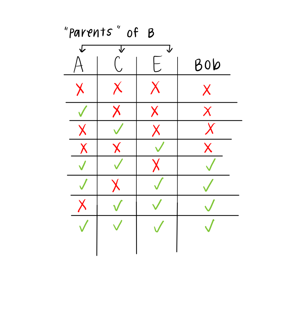
To figure it out, we can make what’s called a truth table, shown above. For each combination of “going” and “not going” that Anna, Carrie, and Erin can have (8 combinations, since they each have 2 choices and 2 x 2 x 2 = 8), we can use Bob’s “rule” to figure out what he will decide. For example, if none of his friends are going (first row), Bob will not go. If all of his friends are going (last row), Bob will go to the party.
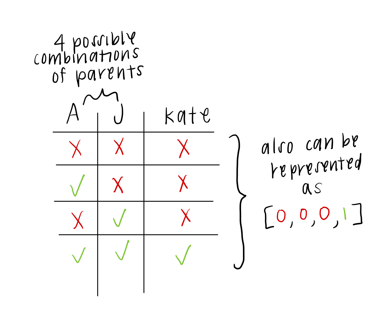
We can technically make this kind of table for each person in our network. Then all we have to do is figure out what the parents of each person are doing, and we can figure out if anyone changes their mind from whatever they initially desired. Furthermore, we can rewrite these rules (if we felt so inclined) as Boolean functions, which only make the rule sound more technical (and easier to understand mathematically, such as for a computer) by using and, or, and not.** For example, Kate’s rule is that she will go if both her friends, John and Anna, are going. We could also say that Kate’s decision is dependent on John and Anna, or KATE = JOHN AND ANNA. The truth table for Kate (or any and function) would look like this:
Every one of our rules can be rewritten as a Boolean function, although some look a bit complicated. Try writing out the truth tables for C = A OR B, C = A AND NOT B, and C = (NOT A) OR C. Keep in mind that “or” in Boolean logic means “at least one of the other, including both.”
We’re getting close to being able to solve our puzzle! We just need to talk about one more thing– how to update someone’s decision based on what their friends are doing. This is where initial conditions will come in. To see how this works, let’s once again look at a simpler problem. We’re going to consider the small network below, with the rules shown below it written in math!
To clarify this network picture a little bit, let’s make a wiring diagram. We’re going to write the three nodes before updating and the three nodes after updating. This means that each person’s decision is based on what their friends have previously decided. For example, Bob’s friends may have already decided not to go, so he won’t go. If Bob’s friends change their mind, the top of the wiring diagram would change, and the bottom would reflect the change in Bob’s decision in response to his friends’ decisions. A little tricky, huh? It looks like this:
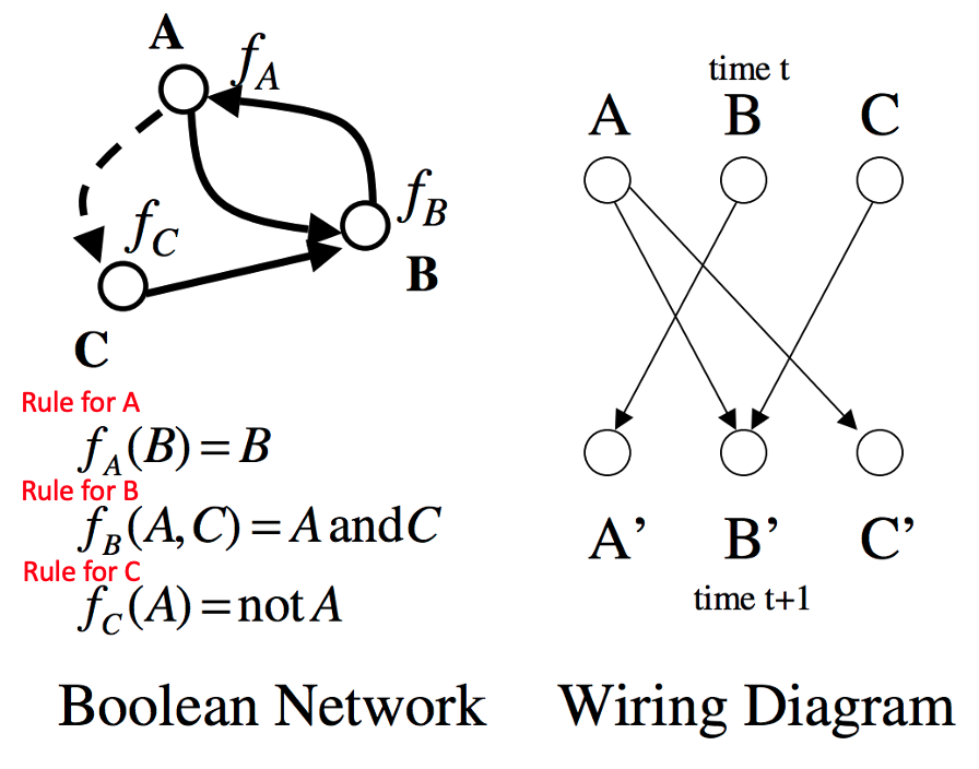
Using the rules for each node, we can also make a truth table for the entire network. In this case, we have condensed three truth tables into one, where the initial state of the three nodes determines the subsequent state of all three nodes. For example, let’s look at “State 1” in the table. A only turns on if B is on (the rule for A above is fA = B), so A will remain off since B is off. B turns on if A and C are both on, so it stays off as well. C turns on when A is off, so it indeed will turn on at this time. We can follow the same logic for the other initial states, and fill out this entire table.

Lastly, we are going to make a state transition graph. Even though this looks like a network, don’t confuse it with the Boolean network above. Here, each node in the network is a different state, meaning each single node represents one state of the entire Boolean network. In this state transition graph, we’re going to draw out how to update the state based on the defined rules. For example, if we are ever in state 1 aka [0,0,0] in this smaller network, we know we will move to state 2 aka [0,0,1]. When we then look at that state in the second row of the truth table, we see something interesting: we stay in state [0,0,1]! Aha! We’ve reached an attractor, giving us the solution for this network if we start from [0,0,0].
What if we start from state 8, [1,1,1]? If you follow the same logic, you’ll find that we eventually end up in the same attractor as before, state 2 aka [0,0,1]. The state transition graph makes this clear:

Interestingly, if we start in state 4, 6, or 3, we end up cycling between states 6 and 3 for eternity. This is a cyclic attractor.
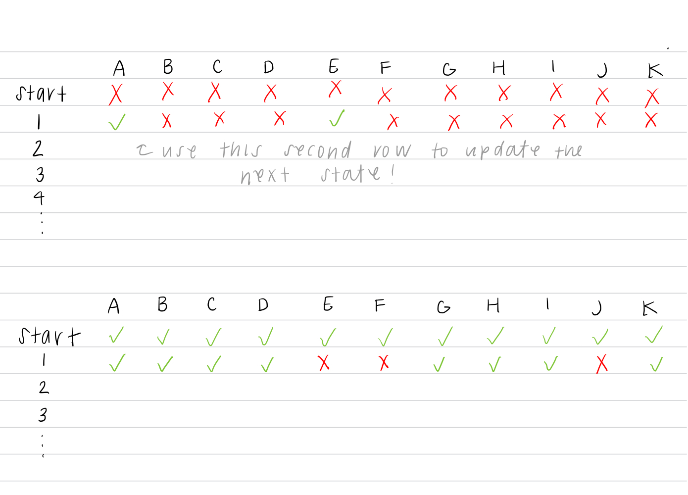
Finally, back to our puzzle! Do you think you have the tools to solve it? Since there are so many people, there are a lot of possible initial conditions, and the state transition graph will be very large. However, we can still consider a few starting states: who goes to the party when no one wants to go initially, and who goes when everyone initially wants to go?
Use the two tables below to fill in each additional row until you reach a stable attractor. That’s your solution! Make sure at each step, you reference the friends’ decisions in the previous row, not the current row. Good luck!
Next post, I’ll talk about how we actually figure out the rules in the first place when we are talking about transcription factor networks.
* An interesting (yet somewhat debated) fact about biological networks is that they tend to be “scale-free.” Scale-invariance is a property meaning that the underlying structure of the network doesn’t change as the network grows. In scale-free networks, you will find that the distribution of edges connected to each node follows a power-law distribution. In simpler terms, this means that are there many nodes with only a few connections, and few nodes with many connections. This is true of airports (Atlanta is one of those few highly-connected nodes) and social networks (there are usually a few well-connected people), but also critical in biological networks where a few nodes have much more control than average. A great visualization of this can be found here. Centrality notions like scale-invariance can also have some interesting side effects, like the fact that on average, most people have fewer friends than their friends have.
** If you’re super savvy with this Boolean language stuff, you might also include XOR, which means “exclusive or.” In Boolean language, “or” means something a little different than everyday language; instead of meaning “one or the other, but not both,” it means “at least one or the other, including both.” XOR is what we mean when we say “or” in the English langauge– “one of the other, but not both.”