Expectations and Densities

CDF and PDF

• In the last lecture, we introduced the ECDF $\hat{F}(x)$ and the CDF $F(x)$, and showed that $\mathbb{E}[\hat{F}(x)]=F(x)$
• For a given function to be a distribution function it must be non-decreasing, go to 0 as $x \rightarrow -\infty$, and go to 1 as $x \rightarrow \infty$

CDF TO PMF

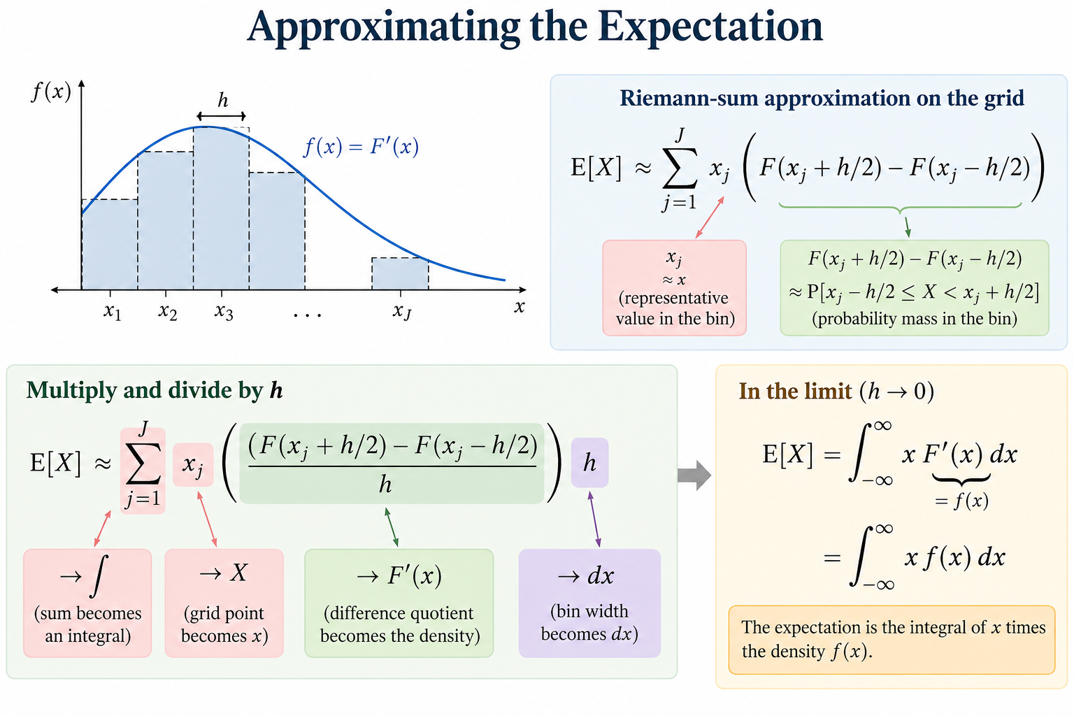
• Let's put $X$ on a grid $\{x_1, x_2, ..., x_J\}$, where the space between $x_j$ and $x_{j+1}$ is $h$
• Let's "split the difference" between grid points, and compute the probability that $X$ is between $x_j - h/2$ and $x_j +h/2$ equal to $F(x_j+h/2) - F(x_j-h/2)$
• Let's approximate the value of $X$ itself on the interval $[x_j-h/2,x_j+h/2)$ by $x_j$
• This discretizes the random variable $X$, giving it a probability mass function and a finite number of values to take

Approximating the Expectation

• On the grid, our approximation of the expected value is $$ \mathbb{E}[X] \approx \sum_{j=1}^J \underbrace{x_j}_{\approx x} \times \underbrace{F(x_j+h/2)-F(x_j-h/2)}_{\approx p[x_j-h/2 \le X < x_j+h]} $$
• We want to let $h$ get small and make this "look like an integral"
• Multiply and divide by $h$, and we get this: $$ \mathbb{E}[X] \approx \underbrace{\sum_{j=1}^J}_{\rightarrow \int} \quad \underbrace{x_j}_{\rightarrow X} \times \underbrace{\frac{F(x_j+h/2)-F(x_j-h/2)}{h}}_{\rightarrow F'(x)} \times \underbrace{h}_{\rightarrow {dx}} $$

PMF to Probability Density Function

• So for a continuous random variable, $$ \mathbb{E}[X] = \int_x x F'(x) dx $$
• The term $F'(x)$ is the probability density function of $F(x)$, and we write $f(x) = F'(x)$
• Some random variables are more easily characterized by their distribution function $F(x)$ (e.g. uniform), and some are more easily characterized by their density $f(x)=F'(x)$ (e.g. normal)

Probability Density Functions

• Some distributions are easier to describe in terms of their density
• Instead of starting with the cdf $F(x)$ and taking the derivative to get the pdf $f(x)=F'(x)$, it makes more sense sometimes to start with the density $f(x)$ and then integrate, so $$ F(x) = \int_{-\infty}^x f(z)dz $$
• Since $F(x) = \text{pr}[ X \le x]$, the complementary probability is $1-F(x) = \text{pr}[X > x]$
• Likewise, $\text{pr}[a \le X < b ] = \int_{a}^{b} f(x)dx = F(b) - F(a)$

Expectation and Variance

• We've defined the expectation and variance a few times, depending on the scenario, but the principles are the same:
  1. To get the expected value, weight each $x$ by the "probability" it occurs, now $f(x)$, and sum
  2. To get the variance, weight each squared deviation of $X$ from its expected value, $(X-\mathbb{E}[X])^2$, by the "probability" it occurs, now $f(x)$, and sum
• With continuous random variables with a density function $f(x)$, we define the expectation as $$ \mathbb{E}[X] = \int_{x} x f(x) dx $$ and the variance as $$ \mathbb{V}[X] = \int_x (x - \mathbb{E}[X])^2 f(x) dx $$

Exercise

• Suppose a variable is uniformly distributed, so it has distribution function: $$ F(x) = \begin{cases} 0, & x < 0 \\ x, & 0 \le x \le 1 \\ 1, & x > 1 \end{cases} $$
• What is the probability density function, the expectation, and variance?

Exercise

• Suppose a variable is exponentially distributed, so it has distribution function: $$ F(x) = \begin{cases} 0, & x < 0 \\ 1-e^{-\lambda t}, & x \ge 0 \end{cases} $$
• What is the probability density function and the expectation?

Distribution Helper

• The next examples use small interactive plots to connect parameters, densities, distribution functions, expectation, and variance
• Move the sliders and watch how the PDF/PMF, CDF, $\mathbb{E}[X]$, and $\mathbb{V}[X]$ change

import numpy as np
import matplotlib.pyplot as plt
from scipy import stats
from scipy.special import gamma
import ipywidgets as widgets


def _format_stat(value):
    if value is None or (isinstance(value, float) and np.isnan(value)):
        return "undefined"
    if np.isposinf(value):
        return "infinite"
    if np.isneginf(value):
        return "-infinite"
    return f"{value:.4g}"


def _finite_grid_from_dist(dist, support=None, q_low=0.001, q_high=0.999, n=600):
    if support is not None:
        lo, hi = support
    else:
        lo = dist.ppf(q_low)
        hi = dist.ppf(q_high)
        if not np.isfinite(lo):
            lo = dist.ppf(0.01)
        if not np.isfinite(hi):
            hi = dist.ppf(0.99)
    if lo == hi:
        lo -= 1
        hi += 1
    pad = 0.04 * (hi - lo)
    return np.linspace(lo - pad, hi + pad, n)


def plot_continuous_distribution(name, dist, mean, variance, support=None):
    x = _finite_grid_from_dist(dist, support=support)
    pdf = dist.pdf(x)
    cdf = dist.cdf(x)

    fig, axes = plt.subplots(1, 2, figsize=(11, 3.8))
    axes[0].plot(x, pdf, color="#2d6cdf", lw=2)
    axes[0].set_title("PDF")
    axes[0].set_xlabel("x")
    axes[0].set_ylabel("f(x)")
    axes[0].grid(alpha=0.25)

    axes[1].plot(x, cdf, color="#00876c", lw=2)
    axes[1].set_title("CDF")
    axes[1].set_xlabel("x")
    axes[1].set_ylabel("F(x)")
    axes[1].set_ylim(-0.04, 1.04)
    axes[1].grid(alpha=0.25)

    if mean is not None and np.isfinite(mean):
        for ax in axes:
            ax.axvline(mean, color="#9f2f2f", ls="--", lw=1.5, label="E[X]")
        axes[0].legend(loc="best")

    # if mean is not None and np.isfinite(mean) and np.isfinite(variance) and variance >= 0:
    #     sd = np.sqrt(variance)
    #     axes[0].axvspan(mean - sd, mean + sd, color="#9f2f2f", alpha=0.10, label="+/- 1 SD")

    fig.suptitle(
        f"{name}: E[X] = {_format_stat(mean)}    V[X] = {_format_stat(variance)}",
        y=1.05,
        fontsize=12,
    )
    plt.tight_layout()
    plt.show()


def plot_discrete_distribution(name, values, probabilities, mean, variance):
    values = np.asarray(values)
    probabilities = np.asarray(probabilities)
    cdf = np.cumsum(probabilities)

    fig, axes = plt.subplots(1, 2, figsize=(11, 3.8))
    axes[0].bar(values, probabilities, color="#2d6cdf", width=0.8)
    axes[0].set_title("PMF")
    axes[0].set_xlabel("x")
    axes[0].set_ylabel("p[X=x]")
    axes[0].grid(axis="y", alpha=0.25)

    axes[1].step(values, cdf, where="post", color="#00876c", lw=2)
    axes[1].scatter(values, cdf, color="#00876c", s=20)
    axes[1].set_title("CDF")
    axes[1].set_xlabel("x")
    axes[1].set_ylabel("F(x)")
    axes[1].set_ylim(-0.04, 1.04)
    axes[1].grid(alpha=0.25)

    if mean is not None and np.isfinite(mean):
        for ax in axes:
            ax.axvline(mean, color="#9f2f2f", ls="--", lw=1.5, label="E[X]")
        axes[0].legend(loc="best")

    fig.suptitle(
        f"{name}: E[X] = {_format_stat(mean)}    V[X] = {_format_stat(variance)}",
        y=1.05,
        fontsize=12,
    )
    plt.tight_layout()
    plt.show()

Example: Uniform

• The uniform distribution spreads probability evenly over an interval $[a,b]$
• Its CDF is $$ F(x) = \begin{cases} 0, & x < a \\ \dfrac{x-a}{b-a}, & a \le x \le b \\ 1, & x > b \end{cases} $$
• Its PDF is $$ f(x) = \begin{cases} \dfrac{1}{b-a}, & a \le x \le b \\ 0, & \text{otherwise} \end{cases} $$

@widgets.interact(
    a=widgets.FloatSlider(value=0.0, min=-5.0, max=5.0, step=0.25, description="a"),
    b=widgets.FloatSlider(value=1.0, min=-4.75, max=10.0, step=0.25, description="b"),
)
def uniform_demo(a, b):
    if b <= a:
        print("Choose b > a.")
        return
    dist = stats.uniform(loc=a, scale=b - a)
    mean = (a + b) / 2
    variance = (b - a) ** 2 / 12
    plot_continuous_distribution("Uniform(a, b)", dist, mean, variance, support=(a, b))

interactive(children=(FloatSlider(value=0.0, description='a', max=5.0, min=-5.0, step=0.25), FloatSlider(value…

Example: The Exponential Distribution

• The exponential distribution is supported on $[0,\infty)$
• Its CDF is $$ F(t) = \begin{cases} 0, & t<0 \\ 1 - e^{-\lambda t}, & t \ge 0 \end{cases} $$
• Its PDF is $$ f(t) = \begin{cases} \lambda e^{-\lambda t}, & t \ge 0 \\ 0, & t<0 \end{cases} $$

@widgets.interact(
    rate=widgets.FloatSlider(value=1.0, min=0.1, max=5.0, step=0.1, description="lambda"),
)
def exponential_demo(rate):
    dist = stats.expon(scale=1 / rate)
    mean = 1 / rate
    variance = 1 / rate**2
    plot_continuous_distribution("Exponential(lambda)", dist, mean, variance, support=(0, dist.ppf(0.995)))

interactive(children=(FloatSlider(value=1.0, description='lambda', max=5.0, min=0.1), Output()), _dom_classes=…

Example: The Logistic Distribution

• The logistic distribution has CDF $$ F(x) = \dfrac{1}{1+e^{-(x-\mu)/\sigma}} $$
• Its PDF is $$ f(x) = \dfrac{e^{-(x-\mu)/\sigma}}{\sigma\left(1+e^{-(x-\mu)/\sigma}\right)^2} $$

@widgets.interact(
    mu=widgets.FloatSlider(value=0.0, min=-5.0, max=5.0, step=0.25, description="mu"),
    sigma=widgets.FloatSlider(value=1.0, min=0.2, max=4.0, step=0.1, description="sigma"),
)
def logistic_demo(mu, sigma):
    dist = stats.logistic(loc=mu, scale=sigma)
    mean = mu
    variance = (np.pi**2 * sigma**2) / 3
    plot_continuous_distribution("Logistic(mu, sigma)", dist, mean, variance)

interactive(children=(FloatSlider(value=0.0, description='mu', max=5.0, min=-5.0, step=0.25), FloatSlider(valu…

Example: Normal Distribution

• The normal density is $$ f(x; \mu, \sigma) = \frac{1}{\sqrt{2\pi} \sigma}e^{-(x-\mu)^2/(2\sigma^2)} $$
• The normal CDF has no elementary closed form, so we usually compute it numerically
• Notice that it is bell-shaped and symmetric around $\mu$

@widgets.interact(
    mu=widgets.FloatSlider(value=0.0, min=-5.0, max=5.0, step=0.25, description="mu"),
    sigma=widgets.FloatSlider(value=1.0, min=0.2, max=4.0, step=0.1, description="sigma"),
)
def normal_demo(mu, sigma):
    dist = stats.norm(loc=mu, scale=sigma)
    mean = mu
    variance = sigma**2
    plot_continuous_distribution("Normal(mu, sigma)", dist, mean, variance)

interactive(children=(FloatSlider(value=0.0, description='mu', max=5.0, min=-5.0, step=0.25), FloatSlider(valu…

Example: Beta Distribution

• The beta distribution is supported on $[0,1]$, so it is useful for probabilities, proportions, and rates
• Its PDF is $$ f(x;\alpha,\beta)=\frac{x^{\alpha-1}(1-x)^{\beta-1}}{B(\alpha,\beta)}, \qquad 0<x<1 $$
• Its CDF does not have a simple closed form for general $\alpha$ and $\beta$

@widgets.interact(
    alpha=widgets.FloatSlider(value=2.0, min=0.2, max=10.0, step=0.2, description="alpha"),
    beta=widgets.FloatSlider(value=2.0, min=0.2, max=10.0, step=0.2, description="beta"),
)
def beta_demo(alpha, beta):
    dist = stats.beta(a=alpha, b=beta)
    mean = alpha / (alpha + beta)
    variance = alpha * beta / ((alpha + beta) ** 2 * (alpha + beta + 1))
    plot_continuous_distribution("Beta(alpha, beta)", dist, mean, variance, support=(0, 1))

interactive(children=(FloatSlider(value=2.0, description='alpha', max=10.0, min=0.2, step=0.2), FloatSlider(va…

Example: Bernoulli Distribution

• A Bernoulli random variable records one success-or-failure trial
• Its PMF is $$ p[X=x] = p^x(1-p)^{1-x}, \qquad x\in\{0,1\} $$
• Its CDF is $$ F(x)=\begin{cases} 0, & x<0 \\ 1-p, & 0\le x<1 \\ 1, & x\ge 1 \end{cases} $$

@widgets.interact(
    p=widgets.FloatSlider(value=0.5, min=0.0, max=1.0, step=0.01, description="p"),
)
def bernoulli_demo(p):
    values = np.array([0, 1])
    probabilities = np.array([1 - p, p])
    mean = p
    variance = p * (1 - p)
    plot_discrete_distribution("Bernoulli(p)", values, probabilities, mean, variance)

interactive(children=(FloatSlider(value=0.5, description='p', max=1.0, step=0.01), Output()), _dom_classes=('w…

Example: Binomial Distribution

• A binomial random variable counts the number of successes in $n$ independent Bernoulli trials with success probability $p$
• Its PMF is $$ p[X=k]=\binom{n}{k}p^k(1-p)^{n-k}, \qquad k=0,1,\ldots,n $$
• Its CDF is the cumulative sum of the PMF: $$ F(k)=\sum_{j=0}^{\lfloor k \rfloor}\binom{n}{j}p^j(1-p)^{n-j} $$

@widgets.interact(
    n=widgets.IntSlider(value=10, min=1, max=60, step=1, description="n"),
    p=widgets.FloatSlider(value=0.5, min=0.0, max=1.0, step=0.01, description="p"),
)
def binomial_demo(n, p):
    values = np.arange(n + 1)
    dist = stats.binom(n=n, p=p)
    probabilities = dist.pmf(values)
    mean = n * p
    variance = n * p * (1 - p)
    plot_discrete_distribution("Binomial(n, p)", values, probabilities, mean, variance)

interactive(children=(IntSlider(value=10, description='n', max=60, min=1), FloatSlider(value=0.5, description=…

Example: Geometric Distribution

• A geometric random variable records the waiting time until the first success
• Here $T=1$ means the first trial succeeds
• Its PMF is $$ p[T=t]=(1-p)^{t-1}p, \qquad t=1,2,3,\ldots $$
• Its CDF is $$ F(t)=p[T\le t]=1-(1-p)^{\lfloor t \rfloor}, \qquad t\ge 1 $$

@widgets.interact(
    p=widgets.FloatSlider(value=0.3, min=0.02, max=1.0, step=0.01, description="p"),
)
def geometric_demo(p):
    dist = stats.geom(p=p)
    upper = int(max(8, dist.ppf(0.995)))
    values = np.arange(1, upper + 1)
    probabilities = dist.pmf(values)
    mean = 1 / p
    variance = (1 - p) / p**2
    plot_discrete_distribution("Geometric(p)", values, probabilities, mean, variance)

interactive(children=(FloatSlider(value=0.3, description='p', max=1.0, min=0.02, step=0.01), Output()), _dom_c…

Example: Poisson Distribution for Count Data

• A Poisson random variable counts how many events occur in a fixed interval when events arrive at average rate $\lambda$
• Its PMF is $$ p[X=k]=e^{-\lambda}\frac{\lambda^k}{k!}, \qquad k=0,1,2,\ldots $$
• Its CDF is the cumulative sum of the PMF: $$ F(k)=\sum_{j=0}^{\lfloor k \rfloor}e^{-\lambda}\frac{\lambda^j}{j!} $$

@widgets.interact(
    lam=widgets.FloatSlider(value=3.0, min=0.1, max=20.0, step=0.1, description="lambda"),
)
def poisson_demo(lam):
    dist = stats.poisson(mu=lam)
    upper = int(max(8, dist.ppf(0.999)))
    values = np.arange(0, upper + 1)
    probabilities = dist.pmf(values)
    mean = lam
    variance = lam
    plot_discrete_distribution("Poisson(lambda)", values, probabilities, mean, variance)

interactive(children=(FloatSlider(value=3.0, description='lambda', max=20.0, min=0.1), Output()), _dom_classes…

Example: Lognormal Distribution

• A lognormal random variable is positive and right-skewed
• If $\log X \sim N(\mu,\sigma^2)$, then $X$ is lognormally distributed
• Its PDF is $$ f(x;\mu,\sigma)=\frac{1}{x\sigma\sqrt{2\pi}}e^{-(\log x-\mu)^2/(2\sigma^2)}, \qquad x>0 $$
• Its CDF can be written using the standard normal CDF $\Phi$: $$ F(x)=\Phi\left(\frac{\log x-\mu}{\sigma}\right), \qquad x>0 $$

@widgets.interact(
    mu=widgets.FloatSlider(value=0.0, min=-2.0, max=2.0, step=0.1, description="mu"),
    sigma=widgets.FloatSlider(value=0.5, min=0.1, max=2.0, step=0.1, description="sigma"),
)
def lognormal_demo(mu, sigma):
    dist = stats.lognorm(s=sigma, scale=np.exp(mu))
    mean = np.exp(mu + sigma**2 / 2)
    variance = (np.exp(sigma**2) - 1) * np.exp(2 * mu + sigma**2)
    plot_continuous_distribution("Lognormal(mu, sigma)", dist, mean, variance, support=(0, dist.ppf(0.995)))

interactive(children=(FloatSlider(value=0.0, description='mu', max=2.0, min=-2.0), FloatSlider(value=0.5, desc…

Example: Pareto Distribution

• The Pareto distribution is a simple model of heavy-tailed positive quantities
• With minimum value $x_m$ and tail parameter $\alpha$, its CDF is $$ F(x)=\begin{cases} 0, & x<x_m \\ 1-\left(\dfrac{x_m}{x}\right)^\alpha, & x\ge x_m \end{cases} $$
• Its PDF is $$ f(x)=\begin{cases} \dfrac{\alpha x_m^\alpha}{x^{\alpha+1}}, & x\ge x_m \\ 0, & x<x_m \end{cases} $$
• As $\alpha$ gets smaller, rare large values become much more important

@widgets.interact(
    alpha=widgets.FloatSlider(value=3.0, min=1.1, max=8.0, step=0.1, description="alpha"),
    xm=widgets.FloatSlider(value=1.0, min=0.5, max=5.0, step=0.25, description="x_m"),
)
def pareto_demo(alpha, xm):
    dist = stats.pareto(b=alpha, scale=xm)
    mean = alpha * xm / (alpha - 1) if alpha > 1 else np.inf
    variance = alpha * xm**2 / ((alpha - 1) ** 2 * (alpha - 2)) if alpha > 2 else np.inf
    plot_continuous_distribution("Pareto(alpha, x_m)", dist, mean, variance, support=(xm, dist.ppf(0.99)))

interactive(children=(FloatSlider(value=3.0, description='alpha', max=8.0, min=1.1), FloatSlider(value=1.0, de…

Example: Mixture of Normals

• A mixture distribution combines two or more probability models
• For a two-component normal mixture with weight $w$, its PDF is $$ f(x)=w f_1(x)+(1-w)f_2(x) $$ where $f_1$ and $f_2$ are normal densities
• Its CDF is the same weighted average of the component CDFs: $$ F(x)=w F_1(x)+(1-w)F_2(x) $$
• This is a useful way to see that distributions can be multi-peaked even when each component is bell-shaped

@widgets.interact(
    w=widgets.FloatSlider(value=0.5, min=0.0, max=1.0, step=0.01, description="w"),
    mu1=widgets.FloatSlider(value=-2.0, min=-6.0, max=3.0, step=0.25, description="mu1"),
    mu2=widgets.FloatSlider(value=2.0, min=-3.0, max=6.0, step=0.25, description="mu2"),
    sigma1=widgets.FloatSlider(value=1.0, min=0.2, max=3.0, step=0.1, description="sigma1"),
    sigma2=widgets.FloatSlider(value=1.0, min=0.2, max=3.0, step=0.1, description="sigma2"),
)
def normal_mixture_demo(w, mu1, mu2, sigma1, sigma2):
    lo = min(mu1 - 4 * sigma1, mu2 - 4 * sigma2)
    hi = max(mu1 + 4 * sigma1, mu2 + 4 * sigma2)
    x = np.linspace(lo, hi, 700)
    pdf = w * stats.norm.pdf(x, mu1, sigma1) + (1 - w) * stats.norm.pdf(x, mu2, sigma2)
    cdf = w * stats.norm.cdf(x, mu1, sigma1) + (1 - w) * stats.norm.cdf(x, mu2, sigma2)
    mean = w * mu1 + (1 - w) * mu2
    second_moment = w * (sigma1**2 + mu1**2) + (1 - w) * (sigma2**2 + mu2**2)
    variance = second_moment - mean**2

    fig, axes = plt.subplots(1, 2, figsize=(11, 3.8))
    axes[0].plot(x, pdf, color="#2d6cdf", lw=2)
    axes[0].axvline(mean, color="#9f2f2f", ls="--", lw=1.5, label="E[X]")
    axes[0].set_title("PDF")
    axes[0].set_xlabel("x")
    axes[0].set_ylabel("f(x)")
    axes[0].grid(alpha=0.25)
    axes[0].legend(loc="best")

    axes[1].plot(x, cdf, color="#00876c", lw=2)
    axes[1].axvline(mean, color="#9f2f2f", ls="--", lw=1.5)
    axes[1].set_title("CDF")
    axes[1].set_xlabel("x")
    axes[1].set_ylabel("F(x)")
    axes[1].set_ylim(-0.04, 1.04)
    axes[1].grid(alpha=0.25)

    fig.suptitle(
        f"Normal mixture: E[X] = {_format_stat(mean)}    V[X] = {_format_stat(variance)}",
        y=1.05,
        fontsize=12,
    )
    plt.tight_layout()
    plt.show()

interactive(children=(FloatSlider(value=0.5, description='w', max=1.0, step=0.01), FloatSlider(value=-2.0, des…