Categorical Variables

Variable and Process

• Our data are samples
• Those samples of data are realizations of a random variable: A phenomenon occurs, and we observe some features or measurements of it
• Those samples are presumed to come from some data generating process; otherwise, the machine cannot learn any stable patterns
• The concept that connects these is the random variable and expectation: How do we expect the data generating process to behave? What can we learn about the random variable from the data we collect?

1. Binomial Variables

Binomial Variables

• A binomial variable takes the values 0 or 1, depending on whether the underlying outcome took one category took one value (e.g. dead) or another (e.g alive)
• The random variable that takes labels into 0/1 values is called a dummy variable

Example:

import numpy as np 
import matplotlib.pyplot as plt 
import pandas as pd 
import seaborn as sns

df = pd.read_csv('./data/heart_failure_clinical_records_dataset.csv')

df.head()

	age	anaemia	creatinine_phosphokinase	diabetes	ejection_fraction	high_blood_pressure	platelets	serum_creatinine	serum_sodium	sex	smoking	time	DEATH_EVENT
0	75.0	0	582	0	20	1	265000.00	1.9	130	1	0	4	1
1	55.0	0	7861	0	38	0	263358.03	1.1	136	1	0	6	1
2	65.0	0	146	0	20	0	162000.00	1.3	129	1	1	7	1
3	50.0	1	111	0	20	0	210000.00	1.9	137	1	0	7	1
4	65.0	1	160	1	20	0	327000.00	2.7	116	0	0	8	1

sns.histplot(data=df, x='DEATH_EVENT', stat='proportion')

<Axes: xlabel='DEATH_EVENT', ylabel='Proportion'>

SEM = np.sqrt( df['DEATH_EVENT'].var()/df.shape[0])
print(f'The standard error of the sample proportion is: {SEM:.3f}' )
df['DEATH_EVENT'].describe()

The standard error of the sample proportion is: 0.027

count    299.00000
mean       0.32107
std        0.46767
min        0.00000
25%        0.00000
50%        0.00000
75%        1.00000
max        1.00000
Name: DEATH_EVENT, dtype: float64

The Bernoulli Trial and Dummy/Boolean Variables

• How do we model and analyze a variable like this?
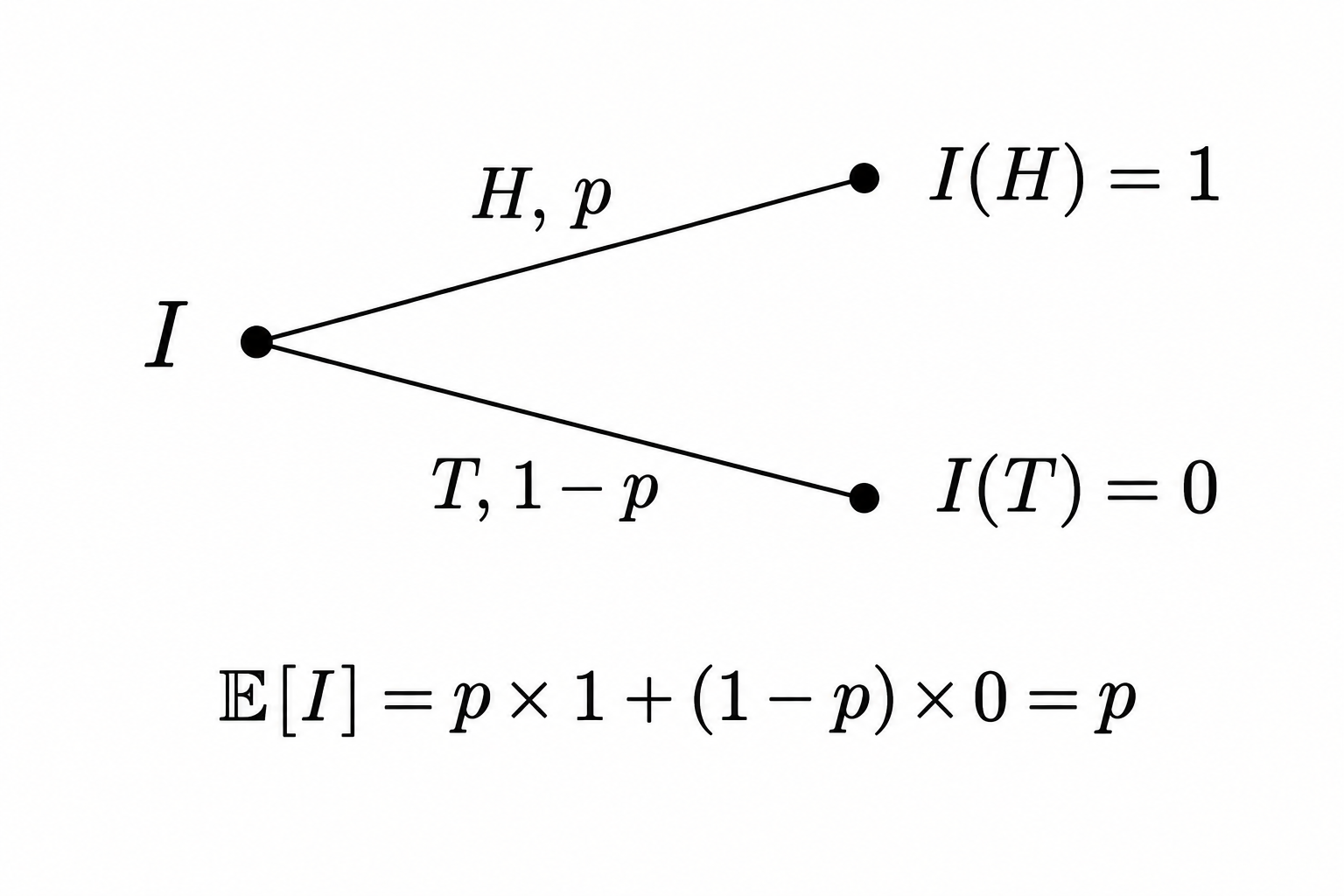
• There are two possible outcomes: $H$ with probability $p$ and $T$ with probability $1-p$
• The random variable $I$ takes $I(H)=1$ for heads and $I(T)=0$ for tails
• We call $I$ an indicator function or dummy variable because it takes the values 0 and 1 depending on whether a condition is true (heads or tails)

Bernoulli Trials: Expectation and Variance

• What is the expectation of this random variable? $$ \mathbb{E}[I] = p \times I(H) + (1-p) \times I(T) = p \times 1 + (1-p) \times 0 = p $$
• Variance? $$ \begin{alignat*}{2} \mathbb{V}[I] &=& \mathbb{E}[ (I - \mathbb{E}[I])^2] \quad(\text{ Definition })\\ &=& p \times (1 - p)^2 + (1-p) \times ( 0 -p)^2 \quad(\text{ Expand defininition })\\ &=& p (1-p) (1-p +p ) \quad(\text{ Factor out $1-p$ })\\ &=& p(1-p) \quad(\text{ Simplify }) \end{alignat*} $$
• For variables with binary outcomes like 0/1, the variance will very often include a term like "$p(1-p)$"

Expectation of the Sample Proportion

• How does a sample of Bernoulli variables behave?
• Since the Bernoulli trial is 0/1-valued, the sample mean is the proportion of observations taking the value 1: $$ \hat{p} = \frac{1}{n} \sum_{i=1}^n I_i, $$ where $I_i=1$ if observation $i$ takes the value 1, and $I_i = 0$ if observation $i$ takes the value 0

• What is the expectations of the sample average? With probability $p$, $I_i = 1$, and with probability $1-p$, $I_i = 0$, so linearity of the expectation implies $$ \begin{alignat*}{2} \mathbb{E}[ \hat{p} ] &=& \mathbb{E}\left[ \frac{1}{n} \sum_{i=1}^n I_i \right] \\ &=& \frac{1}{n} \sum_{i=1}^n \mathbb{E}\left[ I_i \right] \\ &=& \frac{1}{n} \sum_{i=1}^n \left( p \times 1 + (1-p) \times 0 \right) \\ &=& \frac{1}{n} \sum_{i=1}^n p \\ &=& p \end{alignat*} $$
• The expected value of our sample average $\hat{p}$ is equal to the true $p$, and we say that "$\hat{p}$ is an unbiased estimator of $p$"

Categorical Variables/Multinomial Trials

• Imagine there are $L$ possible labels, $\ell_1, \ell_2, ..., \ell_L$
• For example, there are 4 car brands, Honda, Subaru, Ford, and Audi
• The probability of each label, $p_{1}, p_2, ..., p_L$ gives the proportion of the time that each label occurs
• Imagine we are interested in what will happen when, say, the next customer orders a car

Indicator Variables

• For the Bernoulli Trial, we had the indicator labels $I(H) =1$ and $I(T)=0$
• When there is more than one label, we have to be more careful about tracking outcomes
• This concept plays a core role in probability: The indicator function of a categorical $C$ is $$ \mathbb{I}\{ C = \ell \} = \begin{cases} 1, & L = \ell \\ 0, & \text{ otherwise.} \end{cases} $$

Sample Proportion

• How often does a particular label $\ell$ occur in a sample?
• The sample proportion of label $\ell$ is $$ \hat{p}_\ell = \dfrac{1}{N} \sum_{i=1}^N \mathbb{I} \{ c_i = \ell \} $$

Example: Patient Disease from NHAMCS

df = pd.read_csv('./data/ed_visits_probability_lab_train.csv')
df.head()

	sex	arrival_by_ambulance	disease_group	abdominal_pain	cough	vomiting	fever	nausea	chest_pain	shortness_of_breath	...	accident	dizziness	back_pain	anxiety	skin_rash	age_u20	age_20_40	age_40_60	age_60_70	age_o70
0	1	0	cardiovascular	0	0	0	0	0	0	0	...	0	0	0	0	0	1	0	0	0	0
1	1	0	injury_poisoning	1	0	0	0	0	0	0	...	0	0	0	0	0	0	1	0	0	0
2	1	0	dermatologic	0	1	0	0	0	0	0	...	0	0	0	0	1	1	0	0	0	0
3	0	0	other	0	0	0	0	0	0	0	...	0	0	0	0	0	1	0	0	0	0
4	1	0	injury_trauma	0	0	0	0	0	0	0	...	0	0	0	0	0	0	0	1	0	0

5 rows × 21 columns

sns.countplot( y=df['disease_group'] , stat='proportion')

<Axes: xlabel='proportion', ylabel='disease_group'>

Categoricals and One Hot Encoding

• When we create a full set of indicator functions for a labelled variable $C$, we are doing one hot encoding
  • For models with a bias or intercept, you'll typically pd.get_dummies(df[var], dtype=int, drop_first=True) in Pandas, to ensure your variables are not linearly dependent
  • In general, you can pd.get_dummies(df[var], dtype=int)

pd.get_dummies( df['disease_group'], dtype=int)

	cardiovascular	dermatologic	ear_nose_throat_eye	endocrine_metabolic	gastrointestinal	general_constitutional	genitourinary_renal	hepatobiliary_pancreatic	infectious_disease	injury_adverse_care	injury_poisoning	injury_trauma	musculoskeletal	neurological	other	pregnancy_related	psychiatric_behavioral	respiratory
0	1	0	0	0	0	0	0	0	0	0	0	0	0	0	0	0	0	0
1	0	0	0	0	0	0	0	0	0	0	1	0	0	0	0	0	0	0
2	0	1	0	0	0	0	0	0	0	0	0	0	0	0	0	0	0	0
3	0	0	0	0	0	0	0	0	0	0	0	0	0	0	1	0	0	0
4	0	0	0	0	0	0	0	0	0	0	0	1	0	0	0	0	0	0
...	...	...	...	...	...	...	...	...	...	...	...	...	...	...	...	...	...	...
69486	0	0	1	0	0	0	0	0	0	0	0	0	0	0	0	0	0	0
69487	0	0	0	0	1	0	0	0	0	0	0	0	0	0	0	0	0	0
69488	0	0	0	0	0	1	0	0	0	0	0	0	0	0	0	0	0	0
69489	0	0	0	0	0	0	0	0	0	0	0	1	0	0	0	0	0	0
69490	0	0	1	0	0	0	0	0	0	0	0	0	0	0	0	0	0	0

69491 rows × 18 columns

pd.get_dummies( df['disease_group'], dtype=int).mean()

cardiovascular              0.033386
dermatologic                0.026061
ear_nose_throat_eye         0.069074
endocrine_metabolic         0.028953
gastrointestinal            0.056281
general_constitutional      0.115814
genitourinary_renal         0.054626
hepatobiliary_pancreatic    0.008893
infectious_disease          0.042998
injury_adverse_care         0.021744
injury_poisoning            0.011210
injury_trauma               0.254868
musculoskeletal             0.049359
neurological                0.018276
other                       0.085248
pregnancy_related           0.017801
psychiatric_behavioral      0.052338
respiratory                 0.053072
dtype: float64

Properties of the Sample Dummies

• What happens when we take the expectation of the sample proportion? $$ \begin{alignat*}{2} \mathbb{E}\left[ \hat{p}_\ell \right] &=& \mathbb{E}\left[ \frac{1}{n} \sum_{i=1}^n \mathbb{I} \{ C_i = \ell\} \right]\\ &=& \frac{1}{n} \sum_{i=1}^n \mathbb{E}\left[ \mathbb{I} \{ C_i = \ell\} \right] \\ &=& \frac{1}{n} \sum_{i=1}^n p_\ell \\ &=& = p_\ell \end{alignat*} $$
• Since the expectation of $\hat{p}_\ell$ is $p_\ell$, $\hat{p}_\ell$ is an unbiased estimator of $p_\ell$

2. Numeric Variables

Analyzing Numeric Variables

• A numeric variable takes on number values:
  • Real values from $(-\infty, +\infty)$ represented on a computer as a float, like 3.14
  • Integer values from $ ..., -3, -2, -1, 0, 1, 2, 3, ...$ represented on a computer as an int, like 25
• The easiest way to understand what we do today is to ask the question, "How do we analyze numeric variables, as if they were categorical?"

Visualizing Numeric Variables

• For categorical variables, every label occurs many times; for numeric data, a value might occur only once, and many values might be very sparse
• To see why plotting raw values like isn't helpful, consider the rugplot, sns.rugplot()

df = pd.read_csv('./data/heart_failure_clinical_records_dataset.csv')
df.head()

	age	anaemia	creatinine_phosphokinase	diabetes	ejection_fraction	high_blood_pressure	platelets	serum_creatinine	serum_sodium	sex	smoking	time	DEATH_EVENT
0	75.0	0	582	0	20	1	265000.00	1.9	130	1	0	4	1
1	55.0	0	7861	0	38	0	263358.03	1.1	136	1	0	6	1
2	65.0	0	146	0	20	0	162000.00	1.3	129	1	1	7	1
3	50.0	1	111	0	20	0	210000.00	1.9	137	1	0	7	1
4	65.0	1	160	1	20	0	327000.00	2.7	116	0	0	8	1

sns.rugplot( data=df, x= 'ejection_fraction', 
             hue = 'DEATH_EVENT').set(title='Rugplot: This is not very helpful')

[Text(0.5, 1.0, 'Rugplot: This is not very helpful')]

Indicator Functions

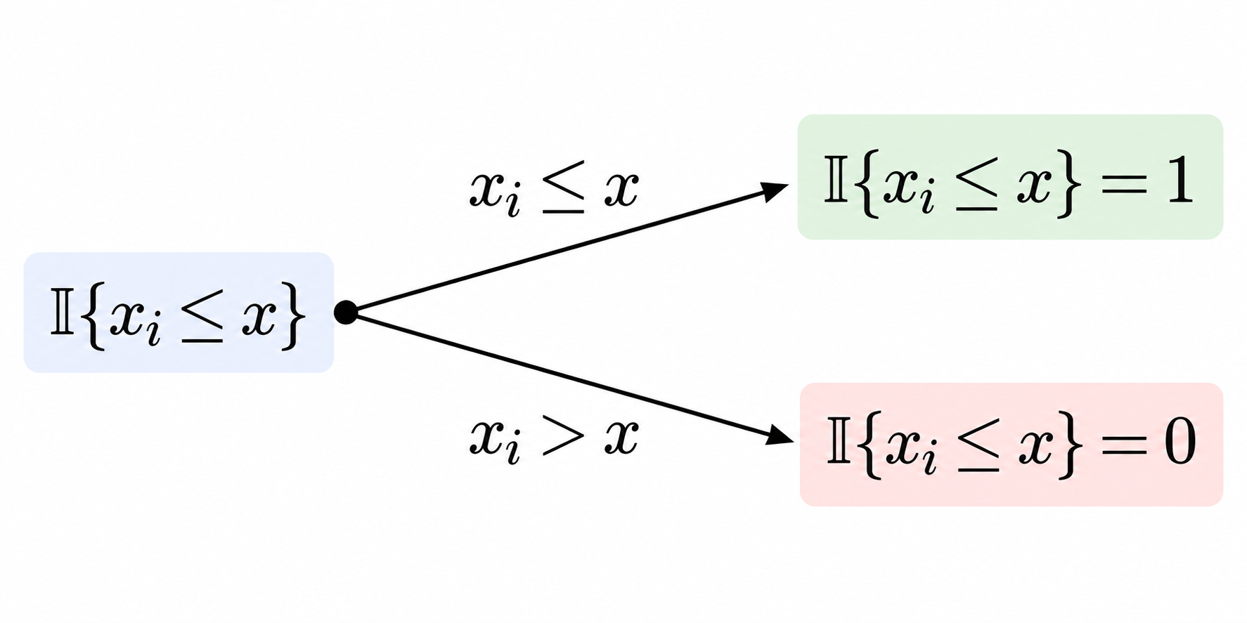
• Imagine we analyze the numeric as if it was a categorical, by sweeping a threshold back and forth, and asking "above or below the threshold?" for each observation
• Instead of asking if the value of the $i$-th observation $x_i$ takes a specific value $x$, we can ask, "Is observation $i$'s value, $x_i$, less than $x$?" $$ \mathbb{I}\{x_i \le x\} = \begin{cases} 1, & x_i \le x\\ 0, & \text{otherwise.} \end{cases} $$

The Empirical Cumulative Distribution Function

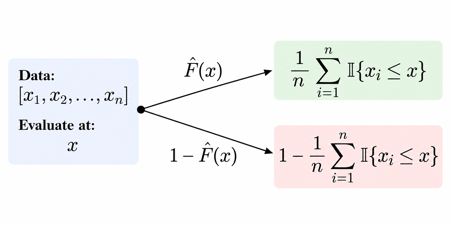
• Now take the sample mean over values $x_i$, and compute the proportion of observations with values less than $x$: $$ \frac{1}{n} \sum_{i=1}^n \mathbb{I} \{x_i \le x\} = \hat{F}(x) $$
• This is like a Bernoulli, where we're asking, "What proportion of the time is $x_i$ is less than $x$?" Or, "If we draw an observation at random, what proportion are above or below $x$?"

Example:

• Suppose your data are [1, 2, 2, 3, 4, 4, 5]
• What is the ECDF?

sns.ecdfplot( data=df, x='ejection_fraction', hue='DEATH_EVENT')

<Axes: xlabel='ejection_fraction', ylabel='Proportion'>

sns.ecdfplot( data=df, x='age', hue='DEATH_EVENT')

<Axes: xlabel='age', ylabel='Proportion'>

sns.ecdfplot( data=df, x='serum_sodium', hue='DEATH_EVENT')

<Axes: xlabel='serum_sodium', ylabel='Proportion'>

The ECDF

• Fix a value $x$. The proportion of the sample $[x_1, x_2, ..., x_n]$ less than $x$ is the function $$ \hat{F}_n(x) = \dfrac{1}{n} \sum_{i=1}^n \mathbb{I}\{x_i \le x\} $$
• This is called the Empirical Cumulative Distribution Function, and is one of our two main ways of modeling a numeric variable

The ECDF

• The ECDF $\hat{F}_X(x)$...
  • must be non-decreasing: As we move $x$ to the right, we capture more observations
  • must be zero as $x$ gets very negative and 1 as $x$ gets very positive: Eventually, all of the sample is above or below the threshold $x$

3. The Cumulative Distribution Function

What is the ECDF Estimating?

• Empirically, the ECDF asks, "What proportion of the data $[x_1, x_2, ..., x_n]$ are below a threshold, $x$?"
• The corresponding population level question is, "What is the probability that the random variable $X$ falls below a threshold, $x$?" $$ F(x) = p[X \le x] $$
• This is the core quantity of probablility: The random variable $X$ turns a probability space $(\mathcal{S}, \mathcal{E}, p)$ into a function we can analyze

The Cumulative Distribution Function

• We define this function as the cumulative distribution function or CDF: $$ F(x) = p[X \le x] = p[ \{ s \text{ in the sample space, such that } X(s)\le x \}] $$
• Notice that, by definition, $\mathbb{E}[ \mathbb{I}\{ X \le x \}] = F(x)$: The expectation of an indicator is the probability the indicator is "on"

The Expected Sample Proportion of the ECDF at a Point

• What is the expected value of the ECDF? $$ \begin{alignat*}{2} \mathbb{E}[\hat{F}(x)] &=& \mathbb{E}_X \left[ \frac{1}{n} \sum_{i=1}^n \mathbb{I} \{ X_i \le x \} \right] \quad \left( \text{ Definition } \right) \\ &=& \frac{1}{n} \sum_{i=1}^n \mathbb{E}_X \left[\mathbb{I} \{ X_i \le x \} \right] \quad \left( \text{Linearity} \right) \\ &=& \frac{1}{n} \sum_{i=1}^n F(x) \quad \left( \text{Expectation of indicator is probability}\right) \\ &=& F(x) \quad \left( \text{Sum of $n$ identical terms over $n$} \right) \end{alignat*} $$
• The ECDF is an unbiased estimator of the true CDF