Random Variables

A Coin Flip

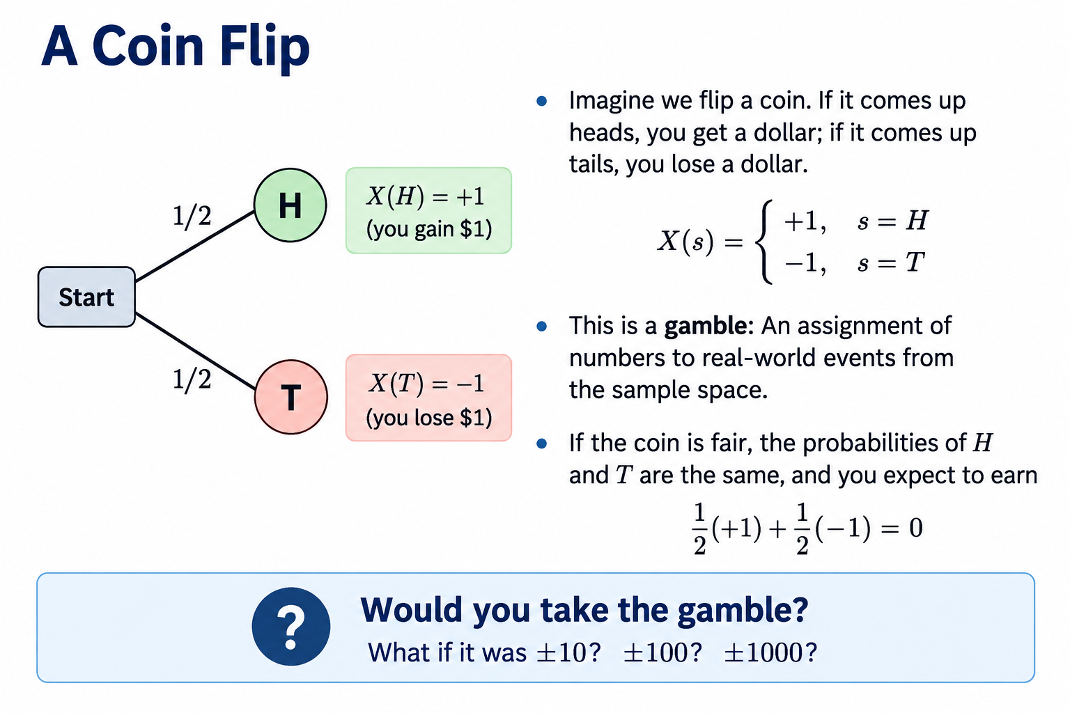
• Imagine we flip a coin. If it comes up heads, you get a dollar; if it comes up tails, you lose a dollar $$ X(s) = \begin{cases} +1, & s = H \\ -1, & s = T \end{cases} $$
• This is a gamble: An assignment of numbers to real-world events from the sample space
• If the coin is fair, the probabilities of $H$ and $T$ are the same, and you expect to earn $\frac{1}{2}(+1)+\frac{1}{2}(-1)=0$
• Would you take the gamble? What if it was $\pm 10$? $\pm 100$? $\pm 1000$?

Review: Probability Spaces

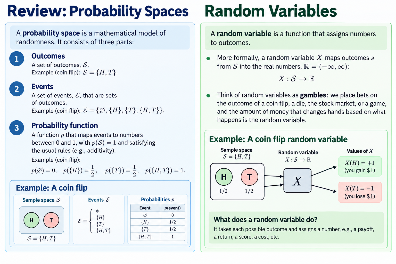
• A probability space is
  1. A set of outcomes, $\mathcal{S}$, like $\mathcal{S} = \{H,T\}$
  2. A set of events, $\mathcal{E}$, that are sets of outcomes, like $\mathcal{E} = \{ \varnothing, H, T, HT \}$
  3. A probability function, $p$, that maps events to numbers between 0 and 1, like $p(\varnothing)=0$, $p(H)=1/2$, $p(T)=1/2$, and $p(HT)=1$

Random Variables

• A random variable is a function $X$ that assigns numbers to outcomes
• More formally, a random variable $X$ maps outcomes $s$ from $\mathcal{S}$ into the real numbers, $\mathbb{R}=(-\infty,\infty)$, or $X : \mathcal{S} \rightarrow \mathbb{R}$
• Think of these as gambles: Let's place bets on the outcome of the die or the stock market or the game, and the amount of money that changes hands based on what happens is the random variable

Random Variables over a Probability Space

• The probability space $(\mathcal{S}, \mathcal{E},p)$ represents our fundamental uncertainty about the world itself: An outcome $s$ in $S$ can be a temperature, an ice cream flavor, a zebra, anything
• The random variable $X$ assigns numbers to those outcomes, like $X(95F)=-6$ or $X(\text{vanilla})=4.25$ or $X(\text{zebra})=23$
• This is where domain expertise matters: What are appropriate numbers to assign to different outcomes?
• There is no "default number" that should be assigned to each outcome; this is a modeling decision. You pick a scale, and that choice determines downstream calculations (E and V).

Probability Mass Functions

• Once we've picked a random variable and make the assignment of outcomes to numbers, we can ask, "What is the probability that $X$ takes a given numeric value?"
• For each value $x$ that $X$ can take, the probability mass function gives $p[ X = x ]$
• In detail: $p[ X = x ] = p[ \{ \text{ every } s \text{ in } \mathcal{S} \text{ such that } X(s) = x \text{ }\}]$
• Notice that if $X$ only takes values $x_1, x_2, ..., x_L$, then $\sum_{\ell = 1}^L p[X=x_\ell] =\sum_{\ell = 1}^L p_\ell = 1$

Key Idea

The state space $\mathcal{S}$ is raw reality, and the random variable $X : \mathcal{S} \rightarrow \mathbb{R}$ turns uncertainty into quantitative analysis

• Once you have a random variable $X$, analysis clicks into place:
  • You can partition the state space by the values $X$ takes on each event-subset (e.g. even vs odd)
  • You don't have to track every conceivable event: Only those events that generate the same values of $X$
  • The probability mass function $p[X=x] = p[ \{ \text{ every } s \text{ in } \mathcal{S} \text{ such that } X(s) = x \text{ }\}]$ are just the probabilities of those events that "matter" with respect to $X$
  • The random variable "pushes" the probability space forward onto the numbers that it takes
• The symbol $X$ corresponds to the random variable and $x$ to the values it takes, just like $f(x)$ corresponds to the function and $y$ to the values it takes

Example: Die

• Imagine rolling a die, but instead of betting on what face comes up, we bet on whether the outcome is even or odd
• Then the random variable is $$ X(s) = \begin{cases} +1, & \text{ $s$ is odd, you win}\\ -1, & \text{ $s$ is even, you lose}\\ \end{cases} $$
• Then the only events you need for this $X$ are $\varnothing$, $\{1,3,5\}$, $\{2,4,6\}$, and $\{1,2,3,4,5,6\}$, with probabilities 0, 1/2, 1/2, and 1, respectively
• Random variables translate a messy world into quantitative analysis

Example: Prediction Markets

• Polymarket, Kalshi, and others are services in which people essentially gamble on events (geopolitical, geological, intellectual...)
• The underlying probability space is complex: $\{$ The US experiences sovereign default in 18 months $\}$, etc.
• Each participant has different beliefs about relative likelihoods
• The random variables are the bets being placed

Expectation

• Suppose there are only $x_1, x_2, ... , x_L$ numeric values that the random variable $X$ takes
• Each of those then occurs with probability $p_1, p_2, ..., p_L$
• What do we "expect" to happen?
• A pessimist might say $\min \{ x_1, ..., x_L\}$, and an optimist might say $\max \{x_1, ..., x_L\}$
• Something in between is the expectation of $X$ i.e the population average ($\mu$): $$ \mathbb{E}[X] = p_1 x_1 + p_2 x_2 + ... + p_L x_L = \sum_{\ell =1}^L p_\ell x_\ell $$
• We weight each numeric outcome by the probability it occurs, and sum
• If you think of the numeric outcomes as literal masses, the expectation is the center of mass

Expectations are Linear

• Imagine we transformed each value of $X$ by $a + bX$; what is $\mathbb{E}[a+bX]$?
• Then we get $$ \begin{alignat*}{2} \sum_{\ell=1}^L p_\ell ( a + b x_\ell) &=& \sum_{\ell=1}^L ( p_\ell a + b p_\ell x_\ell) \quad \text{(Definition)}\\ & =& \sum_{\ell=1}^L p_\ell a + \sum_{\ell=1}^L p_\ell b x_\ell \quad \text{(Break up sum)}\\ &=& a \sum_{\ell=1}^L p_\ell + b \sum_{\ell=1}^L p_\ell x_\ell \quad \text{(Factor out $a$ and $b$)} \\ \underbrace{ \sum_{\ell=1}^L p_\ell ( a + b x_\ell) }_{\mathbb{E}[a+bX]} &=& a + b \underbrace{\sum_{\ell =1}^L p_\ell x_\ell}_{\mathbb{E}[X]} \quad \text{(Use $\sum_{\ell=1}^L p_\ell =1$)} \end{alignat*} $$
• This means that $$ \mathbb{E}[a+bX] = a + b \mathbb{E}[X], $$ and expectation commutes with linear functions
• Since $\mathbb{E}[X]$ itself is just a number like -11 or 22.3, $\mathbb{E}[ \mathbb{E}[X] ] = \mathbb{E}[X]$

Examples

• What is the expected outcomes of a single die roll?
• What is the expected value of rolling two dice, and summing?
• What is the expected value of the minimum of two die? The maximum?

Variance

• How far do you expect $X$ to be from its expectation?
• The variance of $X$ is the expected value of the squared deviations $(X-\mathbb{E}[X])^2$ of $X$ from its expected value: $$ \mathbb{V}[X] = \mathbb{E}[(X-\mathbb{E}[X])^2] = \sum_{\ell =1}^L p_\ell (x_\ell - \mathbb{E}[X])^2 $$
• This measure how dispersed $X$ is around its expectation
• Why standard deviation squared?

Variance of Transformations

• What is the variance of $Y=a+bX$? $$ \begin{alignat*}{2} \mathbb{V}[Y] &=& \sum_{\ell =1}^L p_\ell (y_\ell - \mathbb{E}[Y])^2 \quad \text{(Definition)}\\ &=& \sum_{\ell =1}^L p_\ell (a + b x_\ell - \mathbb{E}[a+b X])^2 \quad \text{(Insert $Y=a+bX$)}\\ &=& \sum_{\ell =1}^L p_\ell (a + b x_\ell - a - b \mathbb{E}[X])^2 \quad \text{(Use linearity of $\mathbb{E}$)}\\ &=& \sum_{\ell =1}^L p_\ell ( b x_\ell - b \mathbb{E}[X])^2 \quad \text{(Cancel $a$'s)}\\ &=& b^2 \times \sum_{\ell =1}^L p_\ell ( x_\ell - \mathbb{E}[X])^2 \quad \text{(Factor out the $b$)}\\ \mathbb{V}[Y] &=& b^2 \times \mathbb{V}[X] \end{alignat*} $$
• So, $\mathbb{V}[Y] \neq a + b \mathbb{V}[X]$

Variance

• This is a very important computational and statistical trick: $$ \begin{alignat*}{2} \mathbb{V}[X] &=& \mathbb{E}[(X-\mathbb{E}[X])^2] \quad \text{(Definition)} \\ &=& \mathbb{E}[(X^2 - 2X\mathbb{E}[X]+\mathbb{E}[X]^2)] \quad \text{(FOIL)} \\ &=& \mathbb{E}[X^2] - 2\mathbb{E}[X]\mathbb{E}[X]+\mathbb{E}[X]^2 \quad \text{(Linearity)}\\ &=& \mathbb{E}[X^2] - \mathbb{E}[X]^2 \quad \text{(Simplify)}\\ \end{alignat*} $$ so the variance is the expectation of $X$ squared, minus the expectation of $X$, squared

Example of variance

• What is the variance of the outcomes of a single die roll?
• What is the variance of rolling two dice, and summing?
• What is the variance of the minimum of two die? The maximum?

Generating Processes and Samples

• Out there in the world, probability spaces $(\mathcal{S}, \mathcal{E}, p)$ are happening
• When we measure features $X$ of those processes, we create an observation $x_i$ of that random variable
• When we collect a set of observations together, we get a random sample of data
• We estimate or fit models to learn from the sample about the underlying probability space $(\mathcal{S}, \mathcal{E}, p)$ and the random variable $X$, so we can make better predictions and decisions

Example: The Sample Mean

• Recall the sample mean: $$ \bar{X}_n = \frac{1}{n} \sum_{i=1}^n X_i $$
• The sample mean is a random variable itself: The underlying data process data itself is random, and the underlying uncertainty associated with $X_1, X_2, ..., $ creates a probability space for $\bar{X}_n$

Independent and Identically Distributed

• A random sample $X_1, X_2, ..., X_n$ is
  • Independent if the observed value of $X_i$ has no influence on the observed value of $X_j$, when $i \neq j$
  • Identically distributed if every $X_i$ is generated by the same probability space and random variable, with expectation $\mathbb{E}[X_i] = \mathbb{E}[X]$
• If a sample is independent and identically distributed, we say it is iid; we will return to this concept later and explore it in more depth later in class
• In notational terms,
  1. Identically distributed implies that for all observations $i$, $\mathbb{E}[X_i] = \mathbb{E}[X]$, since outcome doesn't depend on observation index
  2. Independent implies that $\mathbb{E}[X_i X_j] =\mathbb{E}[X_i] \mathbb[X_j]$, and $\mathbb{E}[X_i]$ doesn't depend on the realization of any other $X_j$

Expectation of the Sample Mean

• Suppose $(X_1, X_2, ..., X_N)$ is an iid sequence, and the variance of each $X_i$ is the same $\mathbb{V}[X]$
• What value do we expect the sample mean to take? $$ \begin{alignat*}{2} \mathbb{E}[\bar{X}_n] &=& \mathbb{E}\left[ \frac{1}{n} \sum_{i=1}^n X_i \right] \quad (\text{Definition})\\ &=& \frac{1}{n} \sum_{i=1}^n \mathbb{E}[ X_i ] \quad (\text{Linearity of $\mathbb{E}$}) \\ &=& \frac{1}{n} \sum_{i=1}^n \mathbb{E}[X] \quad (\text{IID})\\ &=& \mathbb{E}[X] \quad (\text{Sum of $\mathbb{E}[X]$ taken $n$ times, over $n$ }) \end{alignat*} $$
• The expectation of the sample mean is the true population value, $\mathbb{E}[X]$
• This means that $\bar{X}_n$ is an unbiased estimator of the true expected value: By computing the statistic $\bar{X}_n$, we estimate the population parameter $\mathbb{E}[X]$

Variance of the Sample Mean

• We want to compute the variance of the sample mean: $$ \mathbb{V}[\bar{X}_n] = \mathbb{E} \left[ \left( \dfrac{1}{n} \sum_{i=1}^n X_i - \mathbb{E}[\bar{X}_n]\right)^2 \right] $$
• It's about a page of calculations, but the answer is: $$ \mathbb{V}[\bar{X}_n] = \frac{\mathbb{V}[X]}{n} $$
• In words, it's the underlying variance of the population, divided by sample size
• As sample size $n$ goes up, the sample variance goes down: Large samples deliver more precise estimates, in expectation