Inner Product and Orthogonality

Inner Product

• This is the most fundamental calculation in machine learning
• Take two $n$-vectors $x$ and $y$. The inner product $\langle x,y \rangle$ or dot product $x \cdot y$ of $x$ and $y$ is $$ x \cdot y = x_1 y_1 + x_2 y_2 + ... + x_n y_n = \sum_{i=1}^n x_i y_i = x^{\top}y $$
• With numpy, we can use np.inner(x,y) or x @ y
• The inner product creates the shape of space

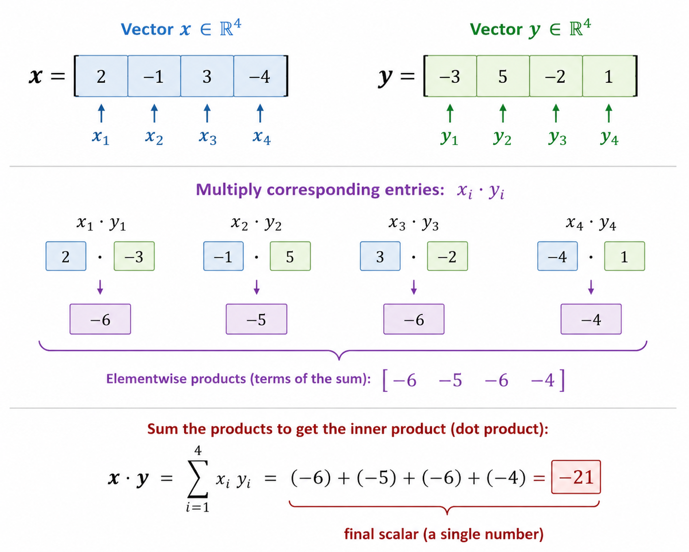
Example 1

Suppose $$ x = \left[ \begin{array}{c} -2 \\ 3 \\ 1 \end{array} \right] \quad \text{and} \quad y = \left[ \begin{array}{c} 1 \\ -1 \\ 2 \end{array} \right]. $$ What is $x \cdot y$?

Length

• The inner product creates the length of a vector
• The length of a vector $x$ is given by $$ ||x|| = \sqrt{x_1^2 + x_2^2 + ... + x_n^2} = \sqrt{\sum_{i=1}^n x_i^2} = \sqrt{x \cdot x } $$
• In numpy, np.sqrt( np.inner(x,x) ) or np.sqrt( x @ x)
• This generalizes absolute value, $|x|=\sqrt{x^2}$

Distance

• The inner product creates distance between points in space
• If length is $||x||$, then the length of the difference between two vectors is distance: $$ ||x-y|| = \sqrt{(x-y) \cdot (x-y) } = \sqrt{\sum_{i=1}^N (x_i-y_i)^2} $$
• In numpy, np.sqrt( ( (x-y) ** 2 ).sum() ) or np.sqrt( np.inner( x-y, x-y) ) or np.sqrt( (x-y) @ (x-y) )
• This generalizes $|x-y|=\sqrt{(x-y)^2}$

Covariance

• Consider two variables $X = (x_1, x_2, ..., x_N)$ and $Y = (y_1, y_2, ..., y_N)$. Center the variables, so $c_X = X-m(X)$ and $c_Y = Y-m(Y)$.
• Then the covariance between $X$ and $Y$, is $$ \text{cov}(X,Y) = \dfrac{\sum_{i=1}^N (x_i - m(X))(y_i - m(Y))}{N} = \dfrac{c_X \cdot c_Y}{N} $$
• If covariance is positive, $X$ tends to be high relative to its mean when $Y$ is high relative to its mean; if covariance is negative, $X$ tends to be high relative to its mean when $Y$ is low relative to its mean
• If covariance is zero, $X$ gives no (linear trend) information about $Y$ and vice versa

Example: Numerical Covariance

Let $X=[1,2,3]^\top$ and $Y=[2,0,4]^\top$. Both variables have mean $2$, so their centered versions are $$ c_X=\left[\begin{array}{c}-1\\0\\1\end{array}\right], \qquad c_Y=\left[\begin{array}{c}0\\-2\\2\end{array}\right]. $$ Their centered dot product is $$ c_X\cdot c_Y=(-1)(0)+(0)(-2)+(1)(2)=2. $$ Therefore, $$ \operatorname{cov}(X,Y)=\frac{c_X\cdot c_Y}{3}=\frac{2}{3}. $$ The positive covariance says that observations above the mean of $X$ tend to occur with observations above the mean of $Y$.

Orthogonality

• If $x \cdot y = 0$, then $x$ and $y$ are orthogonal
• This concept is central to supervised and unsupervised learning (independence of random variables, optimality conditions for regressors, PCA, exclusion restrictions in causal estimation, etc.)
• This is going to be one of the key mathematical concepts you return to over and over

DS Applications of Inner Product

• Covariance is a centered dot product; correlation is a normalized dot product
• Independence implies zero covariance
• Computing the expectation of a random variable: $\mathbb{E}[X] = \sum_{x \in \text{supp}(X)}p(x)x =p \cdot X$
• Solving for the optimal coefficients in a linear regression model: $ X^{\top} \cdot (y - X\beta) = 0$
• Predictions in a linear model are given by $\hat{y}_i = x_i \cdot \beta$
• Testing how similar two documents or images are (cosine similarity of embeddings)
• word2vec and attention are scaled inner products that measure relevance or similarity of tokens
• Deep learning alternates stacked inner product calculations with non-linear activation functions to create complex patterns of learning
• GPUs are expensive because they were developed for computing dot products as fast as possible: Nvidia is a trillion dollar company because of this operation

The key to translating ML concepts effectively to code is, very often, writing vectorized code to optimize dot product calculation or to approximate non-linear operations with a dot product

Example 2

What vectors are orthogonal to $$ x = \left[ \begin{array}{c} -2 \\ 3 \end{array} \right] ? $$ What vectors are orthogonal to $$ y = \left[ \begin{array}{c} -2 \\ 3 \\ 1 \end{array} \right] ? $$

Example 3: Zero Covariance Is Not Independence

Suppose $X$ is equally likely to be $-1$, $0$, or $1$, and let $Y=X^2$. In the three equally likely cases, $$ X=\left[\begin{array}{c}-1\\0\\1\end{array}\right], \qquad Y=\left[\begin{array}{c}1\\0\\1\end{array}\right]. $$ Here $m(X)=0$ and $m(Y)=\frac{2}{3}$, so $$ c_X=\left[\begin{array}{c}-1\\0\\1\end{array}\right], \qquad c_Y=\left[\begin{array}{c}\frac13\\-\frac23\\\frac13\end{array}\right]. $$ What is the centered dot product? Are $X$ and $Y$ independent?

Example 4

• Suppose you have data: A vector $y$ of outcomes and a vector $x$ of explanatory values
• Your predictive model is $\hat{y}_i = b x_i$
• The error term is $e_i = y_i - \hat{y}_i = y_i - b x_i$
• The sum of squared error (SSE) is $\sum_{i=1}^n e_i^2$

1. Show that the SSE is $e \cdot e$
2. Show that the optimal choice of $b$ satisfies $(y-bx) \cdot x = 0$, which is $e \cdot x = 0$: The error and explanatory variable are orthogonal
3. Show that the optimal choice of $b$ is $ x \cdot y / x \cdot x$

Matrix Multiplication

• Matrix multiplication is just an efficient way of "stacking" inner product calculations
• Remember, matrix multiplication is "row times column": That multiplication is a dot product
• This is why $A \times B = C $ requires that $A$ be $(N \times M)$ and $B$ be $(M \times L)$ and you end up with an $(N \times L)$ matrix $C$: The multiplication of each row of length $M$ in $A$ requires that each column be of length $M$ in $B$, and this results in $N$ rows times $L$ columns

Matrix Notation Shortcuts

• Let's write our matrices as $$ A = \left[ \begin{array}{cccc} a_{11} & a_{12} & \dots & a_{1m} \\ a_{21} & a_{22} & \dots & a_{2m} \\ \vdots \\ a_{n1} & a_{n2} & \dots & a_{nm} \\ \end{array} \right] $$ and let the $r$-th row A[r,:] be $$ a_{r,:} = \left[ \begin{array}{cccc}a_{21} & a_{22} & \dots & a_{2m} \end{array} \right] $$ and the $c$-th column A[:,c] be $$ a_{:,c} = \left[ \begin{array}{cccc} a_{1c} \\ a_{2c} \\ \vdots \\ a_{nc} \\ \end{array} \right] $$

Transpose and Identity Matrices

• The transpose of a matrix swaps its rows and columns. If $A$ has entry $a_{ij}$ in row $i$ and column $j$, then $$ (A^\top)_{ij}=a_{ji}. $$ For example, $$ A=\left[\begin{array}{ccc}1 & 2 & 3\\4 & 5 & 6\end{array}\right] \qquad\Longrightarrow\qquad A^\top=\left[\begin{array}{cc}1 & 4\\2 & 5\\3 & 6\end{array}\right]. $$
• The identity matrix $I_n$ is the $n\times n$ matrix with ones on the diagonal and zeroes elsewhere. It acts like the number $1$ in matrix multiplication: $$ I_nx=x, \qquad I_nA=A, \qquad AI_m=A $$ when the dimensions conform. In NumPy, use A.T for a transpose and np.eye(n) for $I_n$.

Matrix-times-Vector

• In this case, compute the inner products of each row of $A$ with the column vector $x$: $$ Ax = \left[ \begin{array}{cccc} a_{11} & a_{12} & \dots & a_{1m} \\ a_{21} & a_{22} & \dots & a_{2m} \\ \vdots \\ a_{n1} & a_{n2} & \dots & a_{nm} \\ \end{array} \right]\left[ \begin{array}{c} x_1 \\ x_2 \\ \vdots \\ x_m \end{array} \right] = \left[ \begin{array}{c} \sum_{j=1}^m a_{1j}x_j \\ \sum_{j=1}^m a_{2j}x_j \\ \vdots \\ \sum_{j=1}^m a_{nj}x_j \end{array} \right] =\left[ \begin{array}{c} a_{1,:}\cdot x \\ a_{2,:}\cdot x \\ \vdots \\ a_{n,:}\cdot x \end{array} \right] $$
• Notice, for this calculation to make sense, $A$ must have $m$ columns, the same as the length of $x$, and the result is an $n$-length vector
• In Numpy, this operation is A@x or np.matmul(A,x), not A*x

Example: Solving Linear Equations with a Matrix

Consider the system $$ 2x_1+x_2=5, \qquad x_1+3x_2=5. $$ We can write it as $Ax=b$, where $$ A=\left[\begin{array}{cc}2 & 1\\1 & 3\end{array}\right], \qquad x=\left[\begin{array}{c}x_1\\x_2\end{array}\right], \qquad b=\left[\begin{array}{c}5\\5\end{array}\right]. $$ Find the $x_1$ and $x_2$ that solve the system.

Matrix-times-Matrix

• Multiplying an $n\times m$ matrix $A$ times an $m \times \ell$ matrix $B$ is the same kind of "row times column" operation, and yields an $n \times \ell$ matrix: $$ AB = \left[ \begin{array}{cccc} a_{11} & a_{12} & \dots & a_{1m} \\ a_{21} & a_{22} & \dots & a_{2m} \\ \vdots \\ a_{n1} & a_{n2} & \dots & a_{nm} \\ \end{array} \right] \left[ \begin{array}{cccc} b_{11} & b_{12} & \dots & b_{1\ell} \\ b_{21} & b_{22} & \dots & b_{2\ell} \\ \vdots \\ b_{m1} & b_{m2} & \dots & b_{m\ell} \\ \end{array} \right] = \left[ \begin{array}{cccc} \sum_{i=1}^m a_{1i}b_{i1} & \sum_{i=1}^m a_{1i}b_{i2} & \dots & \sum_{i=1}^m a_{1i}b_{i\ell} \\ \sum_{i=1}^m a_{2i}b_{i1} & \sum_{i=1}^m a_{2i}b_{i2} & \dots & \sum_{i=1}^m a_{2i}b_{i\ell} \\ \vdots \\ \sum_{i=1}^m a_{ni}b_{i1} & \sum_{i=1}^m a_{ni}b_{i2} & \dots & \sum_{i=1}^m a_{ni}b_{i\ell} \\ \end{array} \right] $$
• This is, of course, A@B or np.matmul(A,B)

Matrix-times-Matrix

• Another way to think about this is: $$ A\cdot B = \left[ \begin{array}{cccc} a_{1,:} \cdot b_{:,1} & a_{1,:} \cdot b_{:,2} & \dots & a_{1,:} \cdot b_{:,\ell} \\ a_{2,:} \cdot b_{:,1} & a_{2,:} \cdot b_{:,2} & \dots & a_{2,:} \cdot b_{:,\ell} \\ \vdots \\ a_{n,:} \cdot b_{:,1} & a_{n,:} \cdot b_{:,2} & \dots & a_{n,:} \cdot b_{:,\ell} \\ \end{array} \right] $$

Example: Non-Square Matrix Multiplication

Let $$ A=\left[\begin{array}{ccc}1 & 2 & 3\\4 & 5 & 6\end{array}\right] \quad (2\times3), \qquad B=\left[\begin{array}{cc}1 & 0\\0 & 1\\1 & 1\end{array}\right] \quad (3\times2). $$

Compute $A \cdot B$. Can you compute $B \cdot A$? First predict its shape, then calculate it. Is it the same matrix as $A\cdot B$?

Example: Adjacency Matrices

Imagine a transportation system, like DC's subway network. We model it as a graph: Each station is a node and if you can go directly from station $i$ to station $j$, the two nodes are adjacent.

An adjacency matrix has entries $$ A_{ij} = \begin{cases} 1, & \text{$i$ and $j$ are connected}\\ 0, & \text{$i$ and $j$ are not connected} \end{cases} $$

Example: Adjacency Matrices

• a. Create the matrix $A$ if the nodes are $a$, $b$, $c$, and $d$ and the undirected edges are $$ \{\{a,c\},\{b,c\},\{b,d\}\}. $$
• b. Notice that if you wanted to get from station $i$ to $k$, that requires that $a_{ij}=1$ and $a_{jk}=1$. Show that $$ A \cdot A = A^2 $$ computes all of these links for you: The $ik$ entry in $A^2$ counts the number of two-step walks from node $i$ to node $k$. Compute $A^2$ for the example.

Advanced Example: Quadratic Forms

Notice that a matrix times a vector is a vector. A vector times a vector is a scalar. Consider the quadratic form

$$ \left[ \begin{array}{cc} x_1 & x_2 \end{array} \right] \left[ \begin{array}{cc} b_{11} & b_{12} \\ b_{21} & b_{22} \end{array} \right] \cdot \left[ \begin{array}{c} x_1 \\ x_2 \end{array} \right] = x^{\top} B x $$

• a. Compute $x^{\top} B x$.
• b. In one dimension, a linear function is $ax$ and a quadratic function is $ax + \frac{b}{2}x^2$. Compute the first and second derivatives of these with respect to $x$.
• c. In two dimensions, a linear function is $a_1 x_1 + a_2 x_2 = a \cdot x$ and a quadratic function is $a \cdot x + \frac{1}{2} x^{\top} B x$. Compute the first and second partial derivatives of these with respect to $x_1$ and $x_2$ and all the pairs of variables.

Advanced Example: Quadratic Forms

• d. In general, for a function $f$ that maps $(x_1,x_2)$ to a number $y$, the Hessian is defined as the matrix of second and cross-partial derivatives of $f$: $$ H = \left[ \begin{array}{cc} \frac{\partial^2 f(x_1, x_2)}{\partial x_1^2} & \frac{\partial^2 f(x_1, x_2)}{\partial x_1 \partial x_2} \\ \frac{\partial^2 f(x_1, x_2)}{\partial x_2 \partial x_1} & \frac{\partial^2 f(x_1, x_2)}{\partial x_2^2} \end{array} \right] $$ Show that the Hessian of $a \cdot x + \frac{1}{2}x^{\top}Bx$ is $\frac{1}{2}(B+B^{\top})$. Conclude that if $B$ is symmetric, the Hessian is $B$.